Freeing a bundle for radiography
A radiograph of an imploding capsule needs a backlighter, and on NIF the backlighter's lasers come out of the drive. Freeing one bundle (two quads of four beams, one quad in each hemisphere, sharing an amplifier chain) leaves 46 quads to drive the hohlraum, and the capsule sees the asymmetry of the missing ports. On a layered DT ignition shot there is little margin for it. A mode-1 asymmetry of the drive, a flux difference between opposite sides of the capsule, pushes the hot spot sideways at about 100 km/s for each percent of mode-1 flux (MacGowan et al., High Energy Density Physics 40, 100944, 2021), and the drive itself is the scarcest resource of the shot.
Which bundle can be freed is set first by the radiograph: its quads must reach a backlighter foil placed across the target from the detector, perpendicular to the line of sight, without their light touching the hohlraum on the way. This tutorial finds the bundles that can serve each of two equatorial lines of sight, ranks them by the symmetry they cost, and compares three ways to win that symmetry back: freeing the bundle's symmetric partner as well, rebalancing the powers of the remaining quads, and re-pointing them within the clearance the entrance holes allow. It introduces three-dimensional mode analysis with real spherical harmonics, the symmetry of the NIF ports, scenarios on a subset of the beams, the influence matrix, optimization with automatic-differentiation gradients, and beam-clearance checks.
using Briareus
using CairoMakie
using LinearAlgebra
using Printf
CairoMakie.activate!(type = "png", px_per_unit = 2)
include(joinpath(pkgdir(Briareus), "docs", "literate", "_plotting.jl"))   # figure helpers
cutaway! (generic function with 1 method)Modes on the capsule
Expand the incident flux on the capsule in real spherical harmonics,
\[H(\theta, \phi) = \sum_{l, m} c_{lm}\, Y_{lm}(\theta, \phi),\]
where $Y_{lm}$ with $m > 0$ varies as $\cos m\phi$ and with $m < 0$ as $\sin |m|\phi$; $Y_{11}$ points along $+x$ and $Y_{1,-1}$ along $+y$. flux_ylm returns the coefficients, in the order of mode_index. The size of mode $l$ relative to the mean is
\[\epsilon_l = \frac{1}{c_{00}}\sqrt{(2l + 1)\sum_m c_{lm}^2},\]
computed by mode_amplitude. For a field with azimuthal symmetry about any axis this is the familiar Legendre ratio $|a_l/a_0|$; for $l = 1$ it is the fractional amplitude $\epsilon$ of a flux $1 + \epsilon\cos\gamma$, where $\gamma$ is the angle from the direction of the asymmetry.
The hohlraum and its pointing
The hohlraum is 10.1 mm long with a radius of 2.875 mm and 3.1 mm laser entrance holes, around a capsule of radius 0.9 mm. Its wall, end caps, entrance holes and capsule carry their exact cylindrical, planar and spherical surfaces (see the Integrating sphere tutorial). nif_quads gives the 48 quads, at 8 TW each, with their measured phase-plate spots. The outer quads are aimed on the hohlraum axis near the entrance-hole planes, at $z = \pm 5.01$ mm (50° cone) and $\pm 5.20$ mm (44.5°); the inner quads at $z = \pm 3.63$ mm (30°) and $\pm 3.09$ mm (23.5°), displaced 0.60 and 1.09 mm from the axis away from their own port, across the hohlraum.
target = hohlraum(length = 10.1, radius = 2.875, leh_radius = 1.55, capsule_radius = 0.9,
                  wall = gold(albedo = 0.85, conversion = 0.8))
pointing = Dict(:outer50 => (0.0, 5.01), :outer44 => (0.0, 5.20),
                :inner30 => (0.60, 3.63), :inner23 => (1.09, 3.09))
function aimed(b)
    r, z = pointing[b.group]
    φ = port_angles(b)[2]
    return remake(b; aim = (-r * cosd(φ), -r * sind(φ), sign(b.port[3]) * z))
end
quads = aimed.(nif_quads(power = 8.0))
48-element Vector{Beam{Float64}}:
Beam(Q15T, θ=23.50°, φ=78.75°, 8 TW, aim=(-0.2126, -1.069, 3.09), defocus=0 mm)
Beam(Q42T, θ=23.50°, φ=168.75°, 8 TW, aim=(1.069, -0.2126, 3.09), defocus=0 mm)
Beam(Q33T, θ=23.50°, φ=258.75°, 8 TW, aim=(0.2126, 1.069, 3.09), defocus=0 mm)
Beam(Q24T, θ=23.50°, φ=348.75°, 8 TW, aim=(-1.069, 0.2126, 3.09), defocus=0 mm)
Beam(Q13T, θ=30.58°, φ=34.33°, 8 TW, aim=(-0.4955, -0.3384, 3.63), defocus=0 mm)
Beam(Q41T, θ=30.00°, φ=123.75°, 8 TW, aim=(0.3333, -0.4989, 3.63), defocus=0 mm)
Beam(Q36T, θ=30.58°, φ=214.33°, 8 TW, aim=(0.4955, 0.3384, 3.63), defocus=0 mm)
Beam(Q26T, θ=30.00°, φ=303.75°, 8 TW, aim=(-0.3333, 0.4989, 3.63), defocus=0 mm)
Beam(Q14T, θ=44.50°, φ=16.29°, 8 TW, aim=(-0, -0, 5.2), defocus=0 mm)
Beam(Q12T, θ=44.50°, φ=62.46°, 8 TW, aim=(-0, -0, 5.2), defocus=0 mm)
⋮
Beam(Q22B, θ=135.50°, φ=343.71°, 8 TW, aim=(-0, 0, -5.2), defocus=0 mm)
Beam(Q16B, θ=150.00°, φ=56.25°, 8 TW, aim=(-0.3333, -0.4989, -3.63), defocus=0 mm)
Beam(Q44B, θ=149.42°, φ=145.67°, 8 TW, aim=(0.4955, -0.3384, -3.63), defocus=0 mm)
Beam(Q31B, θ=150.00°, φ=236.25°, 8 TW, aim=(0.3333, 0.4989, -3.63), defocus=0 mm)
Beam(Q21B, θ=149.42°, φ=325.67°, 8 TW, aim=(-0.4955, 0.3384, -3.63), defocus=0 mm)
Beam(Q15B, θ=156.50°, φ=11.25°, 8 TW, aim=(-1.069, -0.2126, -3.09), defocus=0 mm)
Beam(Q42B, θ=156.50°, φ=101.25°, 8 TW, aim=(0.2126, -1.069, -3.09), defocus=0 mm)
Beam(Q33B, θ=156.50°, φ=191.25°, 8 TW, aim=(1.069, 0.2126, -3.09), defocus=0 mm)
Beam(Q24B, θ=156.50°, φ=281.25°, 8 TW, aim=(-0.2126, 1.069, -3.09), defocus=0 mm)A Scenario holds what does not change while beams are re-aimed and their powers adjusted: the target, the deposition operator for these ports, the view factors, the linear response of the capsule's incident flux to the power each element absorbs, and the mode weights of the capsule. Its parameterization here gives each quad its own power.
The deposition operator is sampled more coarsely than its defaults, to keep the optimizations below quick: points no farther apart than 0.6 of the spot's smaller semi-axis (rather than 0.3), refined only within 0.5 mm of each beam's footprint (rather than 2 mm; no aim moves by more than 0.3 mm here), and one point per triangle elsewhere. That cuts the operator to a fifth of its points and changes the modes below in the fourth digit.
scenario = Scenario(target, quads; observe = :capsule,
                    deposition_kw = (; resolution = 0.6, reach = 0.5, level = 0),
                    parameterization = GroupPointing(quads; by = :quad, fields = (:power,)))
full = flux_ylm(evaluate(scenario, quads); lmax = 4)
show_modes(label, c) = @printf("%-24s ε₁ %6.3f%%  ε₂ %6.3f%%  ε₃ %6.3f%%  ε₄ %6.3f%%  drive %.4f\n",
                               label, (100 * mode_amplitude(c, l) for l in 1:4)..., c[1] / full[1])
show_modes("48 quads", full)
48 quads ε₁ 0.000% ε₂ 14.422% ε₃ 0.208% ε₄ 0.647% drive 1.0000With all 48 quads the drive has the large $l = 2$ asymmetry of this untuned pointing (the cone powers and pointing would tune it away) and no mode 1.
The symmetry of the ports
The NIF ports are not symmetric under every rotation that leaves the hohlraum unchanged. Rotating every port by 180° about the $x$, $y$ or $z$ axis maps the set of ports onto itself, but rotating by 90° about $z$, inverting through the center, or reflecting through the equatorial plane does not:
ports = [b.port for b in quads]
maps_onto_itself(f) = all(any(norm(f(p) - q) < 1e-6 for q in ports) for p in ports)
operations = ["180° about x" => p -> [p[1], -p[2], -p[3]],
              "180° about y" => p -> [-p[1], p[2], -p[3]],
              "180° about z" => p -> [-p[1], -p[2], p[3]],
              "90° about z" => p -> [-p[2], p[1], p[3]],
              "inversion" => p -> -p,
              "reflection in z = 0" => p -> [p[1], p[2], -p[3]]]
for (name, f) in operations
    @printf("%-20s %s\n", name, maps_onto_itself(f) ? "symmetry" : "not a symmetry")
end
180° about x symmetry
180° about y symmetry
180° about z symmetry
90° about z not a symmetry
inversion not a symmetry
reflection in z = 0 not a symmetryThe three rotations form the group $D_2$. A harmonic survives the average over $D_2$ only if each rotation leaves it unchanged. A rotation by 180° about $z$ multiplies $Y_{lm}$ by $(-1)^m$, and one about $x$ multiplies it by $(-1)^{l+m}$ for $m \ge 0$ and by $(-1)^{l+m+1}$ for $m < 0$. A drive with the symmetry of the ports can therefore contain only even $m$, with $l$ even for the cosine harmonics and $l$ odd for the sine harmonics. Every coefficient the rule forbids is zero to round-off:
allowed(l, m) = iseven(m) && (m >= 0 ? iseven(l) : isodd(l))
forbidden = [abs(full[mode_index(l, m)]) for l in 0:4 for m in -l:l if !allowed(l, m)]
@printf("largest forbidden |c_lm|/c₀₀ %.1e\n", maximum(forbidden) / full[1])
for l in 1:4, m in -l:l
    allowed(l, m) && @printf("c(%d,%2d)/c₀₀ = %+.5f\n", l, m, full[mode_index(l, m)] / full[1])
end
largest forbidden |c_lm|/c₀₀ 2.1e-16
c(2, 0)/c₀₀ = -0.06449
c(2, 2)/c₀₀ = -0.00046
c(3,-2)/c₀₀ = +0.00079
c(4, 0)/c₀₀ = +0.00152
c(4, 2)/c₀₀ = -0.00001
c(4, 4)/c₀₀ = -0.00153The cosine $l = 2, m = 2$ and sine $l = 3, m = -2$ harmonics are allowed by the ports' symmetry, and the ports excite them weakly.
Which bundles can drive the backlighter
Two lines of sight at the equator ($\theta = 90°$) suit radiography of the capsule, at $\phi = 78°$ and $\phi = 348°$. For each, a 2 mm backlighter foil faces the detector from the far side of the target, a distance $d$ from the target center; the radiography beams strike its face toward the target, so the x rays they generate cross the capsule to the detector. The "sombrero", the dimpled shield around the entrance hole that keeps unconverted 1ω light off the hohlraum and its thermo-mechanical package, also stands between some beams and the foil; it is not modeled here, so this selection is necessary but not sufficient. A quad can drive the foil if it strikes that face at less than 70° from its normal, the LMF limit for laser capture on a target surface, and if its beam, aimed at the foil center, clears the hohlraum and capsule on the way. The clearance is judged as a shot review judges it, on the worst case: clearance grows each beam's envelope (its contour at 1% of the peak, spread by the f-cone) by 50 µm of pointing error and 25 µm of target positioning, adds ±1 mm of focus error, and reports the smallest distance to the hardware. That distance is exact; only the power on the hardware, not used here, depends on how finely the error set and the spot are sampled, so both are sampled coarsely. The foil's distance is a design choice; two are tried.
function backlighter_bundles(φ_los, d)
    n = [cosd(φ_los), sind(φ_los), 0.0]                    # toward the detector
    center = Tuple(-d .* n)
    scene = Target(target.components..., foil(:backlighter, center, Tuple(n); width = 2.0, n = 8))
    found = []
    for k in sort(collect(keys(bundles)))
        qs = quads[bundles[k]]
        incidence = [acosd(dot(b.port, n)) for b in qs]
        all(<(70), incidence) || continue
        report = clearance(scene, [remake(b; aim = center) for b in qs];
                           targets = (:backlighter,), hardware = (:wall, :cap_top, :cap_bottom, :capsule),
                           peak_fraction = 0.01, wings = [], nangles = 4, nspot = 15)
        push!(found, (bundle = k, incidence, clearance = minimum(r -> r.clearance, report.rows)))
    end
    return found
end

bundles = nif_bundles(quads)
for φ_los in (78.0, 348.0)
    near, far = backlighter_bundles(φ_los, 8.0), backlighter_bundles(φ_los, 12.0)
    @printf("line of sight 90-%g: %d bundles within 70°\n", φ_los, length(near))
    @printf("  %-7s %-16s %-14s %s\n", "bundle", "cones", "incidence", "worst-case clearance, d = 8 / 12 mm")
    for (a, b) in zip(near, far)
        cones = join(sort(unique(string(quads[i].group) for i in bundles[a.bundle])), "+")
        @printf("  %-7s %-16s %4.1f°, %4.1f°   %6.2f / %5.2f mm\n", a.bundle, cones, a.incidence...,
                a.clearance, b.clearance)
    end
end
line of sight 90-78: 6 bundles within 70°
bundle cones incidence worst-case clearance, d = 8 / 12 mm
11 outer50 53.1°, 47.1° -0.62 / 2.04 mm
12 outer44 47.5°, 45.7° -1.01 / 1.67 mm
16 inner30+outer50 40.4°, 62.3° -1.18 / 0.73 mm
41 inner30+outer50 69.6°, 43.1° -1.18 / 1.22 mm
43 outer44 51.9°, 57.3° -0.13 / 2.82 mm
46 outer50 61.4°, 69.2° 1.87 / 4.93 mm
line of sight 90-348: 6 bundles within 70°
bundle cones incidence worst-case clearance, d = 8 / 12 mm
11 outer50 61.6°, 69.4° 1.90 / 4.96 mm
13 inner30+outer50 69.4°, 43.1° -1.18 / 1.22 mm
14 outer44 51.9°, 57.3° -0.13 / 2.82 mm
21 inner30+outer50 40.4°, 61.9° -1.18 / 0.73 mm
22 outer44 47.5°, 45.7° -1.01 / 1.67 mm
23 outer50 53.2°, 47.3° -0.59 / 2.07 mmEach line of sight can be served by six bundles. With the foil 12 mm from the center all six clear the hohlraum; at 8 mm the hohlraum is in the way of all but one, whose quads pass above and below it at steep incidence: bundle 46 for 90-78 and bundle 11 for 90-348. Their lower quads strike the foil at 69°, just inside the capture limit.
What each bundle costs
Without a laser–plasma model the capsule's flux is linear in the beam powers. influence_matrix returns the harmonic coefficients produced by each quad alone at 1 TW, so the coefficients for any assignment of powers $P$ are $M P$. nif_bundles groups the quads into bundles.
M = influence_matrix(scenario, quads; lmax = 4)
P_full = [b.power for b in quads]
without(k) = setdiff(eachindex(quads), bundles[k])
without (generic function with 1 method)The rotations of $D_2$ carry each bundle onto another, so the 24 bundles fall into sets of equivalent bundles, and freeing any member of a set costs the same. Each quad's image under a rotation is a quad of the image bundle:
image(i, f) = findfirst(q -> norm(f(quads[i].port) - q.port) < 1e-6, quads)
rotations = last.(operations[1:3])
image_bundle(k, f) = only(unique(nif_bundle(quads[image(i, f)]) for i in bundles[k]))
orbits = unique(sort(unique([k; [image_bundle(k, f) for f in rotations]])) for k in keys(bundles))

cost(k) = M[:, without(k)] * P_full[without(k)]
sort!(orbits; by = o -> mode_amplitude(cost(o[1]), 1))
@printf("%-13s %-15s %7s %7s %7s %7s %7s\n", "bundles", "cones", "ε₁ (%)", "ε₂ (%)",
        "ε₃ (%)", "ε₄ (%)", "drive")
for o in orbits
    cones = join(sort(unique(string(quads[i].group) for i in bundles[o[1]])), "+")
    ε = [[mode_amplitude(cost(k), l) for l in 1:4] for k in o]
    @assert all(e -> isapprox(e, ε[1]; atol = 1e-9), ε)
    @printf("%-13s %-15s %7.3f %7.3f %7.3f %7.3f %7.4f\n", join(o, " "), cones,
            (100 .* ε[1])..., cost(o[1])[1] / full[1])
end
bundles cones ε₁ (%) ε₂ (%) ε₃ (%) ε₄ (%) drive
11 23 34 46 outer50 1.080 15.267 0.786 0.710 0.9625
14 22 35 45 outer44 1.472 15.091 0.869 0.756 0.9606
12 25 32 43 outer44 1.472 15.082 0.807 0.755 0.9606
15 24 33 42 inner23 2.974 13.374 1.025 0.833 0.9533
13 21 36 44 inner30+outer50 3.073 14.079 1.243 0.519 0.9565
16 26 31 41 inner30+outer50 3.097 14.091 1.182 0.529 0.9566A bundle's two quads need not share a cone. The bundles whose quads both sit in the 50° cone cost least, in mode 1 and in drive, and those of the 44.5° cone next. A bundle with an inner quad costs three times as much mode 1: the inner quads deposit their power around the waist of the hohlraum, closest to the capsule. Among the bundles that can drive a backlighter, the 50° bundles are therefore the ones to free: 11 or 23 for the line of sight at 90-348, 46 or 11 for 90-78, and with the foil at 8 mm only 11 and 46 remain. This tutorial frees bundle 11, the pair Q11T and Q11B, for the line of sight at 90-348; bundle 46 is its image under a rotation of $D_2$ and costs the same.
freed = "11"
keep = without(freed)
remaining = quads[keep]
46-element Vector{Beam{Float64}}:
Beam(Q15T, θ=23.50°, φ=78.75°, 8 TW, aim=(-0.2126, -1.069, 3.09), defocus=0 mm)
Beam(Q42T, θ=23.50°, φ=168.75°, 8 TW, aim=(1.069, -0.2126, 3.09), defocus=0 mm)
Beam(Q33T, θ=23.50°, φ=258.75°, 8 TW, aim=(0.2126, 1.069, 3.09), defocus=0 mm)
Beam(Q24T, θ=23.50°, φ=348.75°, 8 TW, aim=(-1.069, 0.2126, 3.09), defocus=0 mm)
Beam(Q13T, θ=30.58°, φ=34.33°, 8 TW, aim=(-0.4955, -0.3384, 3.63), defocus=0 mm)
Beam(Q41T, θ=30.00°, φ=123.75°, 8 TW, aim=(0.3333, -0.4989, 3.63), defocus=0 mm)
Beam(Q36T, θ=30.58°, φ=214.33°, 8 TW, aim=(0.4955, 0.3384, 3.63), defocus=0 mm)
Beam(Q26T, θ=30.00°, φ=303.75°, 8 TW, aim=(-0.3333, 0.4989, 3.63), defocus=0 mm)
Beam(Q14T, θ=44.50°, φ=16.29°, 8 TW, aim=(-0, -0, 5.2), defocus=0 mm)
Beam(Q12T, θ=44.50°, φ=62.46°, 8 TW, aim=(-0, -0, 5.2), defocus=0 mm)
⋮
Beam(Q22B, θ=135.50°, φ=343.71°, 8 TW, aim=(-0, 0, -5.2), defocus=0 mm)
Beam(Q16B, θ=150.00°, φ=56.25°, 8 TW, aim=(-0.3333, -0.4989, -3.63), defocus=0 mm)
Beam(Q44B, θ=149.42°, φ=145.67°, 8 TW, aim=(0.4955, -0.3384, -3.63), defocus=0 mm)
Beam(Q31B, θ=150.00°, φ=236.25°, 8 TW, aim=(0.3333, 0.4989, -3.63), defocus=0 mm)
Beam(Q21B, θ=149.42°, φ=325.67°, 8 TW, aim=(-0.4955, 0.3384, -3.63), defocus=0 mm)
Beam(Q15B, θ=156.50°, φ=11.25°, 8 TW, aim=(-1.069, -0.2126, -3.09), defocus=0 mm)
Beam(Q42B, θ=156.50°, φ=101.25°, 8 TW, aim=(0.2126, -1.069, -3.09), defocus=0 mm)
Beam(Q33B, θ=156.50°, φ=191.25°, 8 TW, aim=(1.069, 0.2126, -3.09), defocus=0 mm)
Beam(Q24B, θ=156.50°, φ=281.25°, 8 TW, aim=(-0.2126, 1.069, -3.09), defocus=0 mm)Freeing bundle 11
A subset of the scenario holds the 46 remaining quads and reuses everything but the deposition operator, which it restricts to their ports. The same coefficients follow from the full scenario with the bundle's quads at zero power, and from the influence matrix:
c_free = flux_ylm(evaluate(subset(scenario, keep), remaining); lmax = 4)
zeroed = [i in bundles[freed] ? remake(b; power = 0.0) : b for (i, b) in enumerate(quads)]
c_zeroed = flux_ylm(evaluate(scenario, zeroed); lmax = 4)
c_matrix = M[:, keep] * P_full[keep]
@printf("subset vs zero power %.1e   subset vs influence matrix %.1e\n",
        norm(c_free - c_zeroed) / norm(c_free), norm(c_free - c_matrix) / norm(c_free))
show_modes("bundle 11 freed", c_free)
subset vs zero power 0.0e+00 subset vs influence matrix 1.4e-15
bundle 11 freed ε₁ 1.080% ε₂ 15.267% ε₃ 0.786% ε₄ 0.710% drive 0.9625The drive falls by 4% and a mode-1 asymmetry of 1.1% appears, about 110 km/s of hot-spot velocity. Its direction lies between the azimuths of the freed quads' ports:
dipole = normalize([c_free[mode_index(1, 1)], c_free[mode_index(1, -1)], c_free[mode_index(1, 0)]])
@printf("mode-1 direction θ = %.1f°, φ = %.1f°\n", acosd(dipole[3]),
        mod(atand(dipole[2], dipole[1]), 360))
for i in bundles[freed]
    @printf("%s port θ = %.2f°, φ = %.2f°\n", quads[i].name, port_angles(quads[i])...)
end
mode-1 direction θ = 90.0°, φ = 45.1°
Q11T port θ = 50.00°, φ = 39.67°
Q11B port θ = 130.00°, φ = 50.62°An outer quad crosses the hohlraum axis near its entrance hole and heats the wall on the far side, so without it the side of the capsule facing away from its port is colder.
The maps below show the flux on the capsule as seen from outside, in an equal-area (Hammer) projection, so that equal areas of the map are equal solid angles of the capsule. Polar angle θ is marked at the left edge and azimuth φ along the equator, which runs across the middle. The flux is computed per element, on 24 × 32 patches in θ and φ; the maps interpolate it linearly from the patch values averaged onto their corners. The left map shows the flux relative to its own mean, $H/\langle H\rangle - 1$, where $\langle H\rangle = c_{00}/\sqrt{4\pi}$. The right map subtracts the same quantity for all 48 quads, which isolates what freeing the bundle changed. The figure helpers sphere_axis, sphere_map and mark_directions! come from docs/literate/_plotting.jl.
capsule = elements(target, :capsule)
deviation(H, c) = 100 .* (H ./ (c[1] / sqrt(4π)) .- 1)       # percent of ⟨H⟩
H_full = evaluate(scenario, quads).flux
H_free = evaluate(subset(scenario, keep), remaining).flux
port_marker = (marker = :xcross, markersize = 12, color = :black)
los_marker = (marker = :circle, markersize = 11, color = :transparent, strokecolor = :black,
              strokewidth = 1.5)
function capsule_panel(pos, field, range; title = "")
    ax = sphere_axis(pos; title)
    hm = sphere_heatmap!(ax, sphere_map(target, field, :capsule); colormap = :balance,
                         colorrange = (-range, range))
    mark_directions!(ax, [port_angles(quads[i]) for i in bundles[freed]]; port_marker...)
    mark_directions!(ax, [(90, 348)]; los_marker...)
    return hm
end
capsule_legend(pos) = Legend(pos, [MarkerElement(; port_marker...), MarkerElement(; los_marker...)],
                             ["ports of the freed quads", "line of sight 90-348"];
                             orientation = :horizontal, framevisible = false)

fig = Figure(size = (800, 330))
hm = capsule_panel(fig[1, 1], deviation(H_free, c_free), 15; title = "bundle 11 freed")
Colorbar(fig[2, 1], hm; vertical = false, flipaxis = false, width = Relative(0.7),
         label = "H/⟨H⟩ − 1 (%)")
hm = capsule_panel(fig[1, 2], deviation(H_free, c_free) - deviation(H_full, full), 2;
                   title = "change from 48 quads")
Colorbar(fig[2, 2], hm; vertical = false, flipaxis = false, width = Relative(0.7),
         label = "difference in H/⟨H⟩ − 1 (%)")
capsule_legend(fig[3, 1:2])
rowgap!(fig.layout, 6)
fig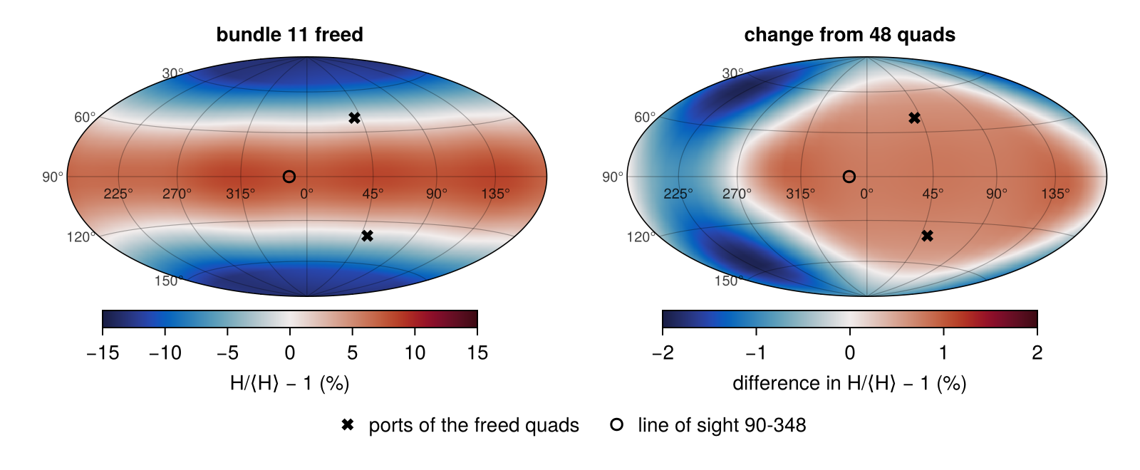
The untuned $l = 2$ asymmetry, a hot waist and cold poles, dominates the flux and barely changes. What freeing the bundle changed is mostly mode 1: the side facing the freed ports, around $\phi = 45°$, is warmer relative to the mean by about 1%, and the far side, where the freed quads deposited their power, colder by up to 2%.
Remedy 1: free the partner as well
The rotation by 180° about $z$ carries bundle 11 onto bundle 34. Freeing both leaves ports with that symmetry, which removes every harmonic of odd $m$, among them the two transverse components of mode 1. The axial component $c_{10}$ vanishes for another reason: the hohlraum is axisymmetric, so a quad's contribution to $c_{10}$ depends only on its cone and hemisphere, and each freed bundle takes one quad from each hemisphere of the same cone.
partner = image_bundle(freed, rotations[3])
keep_pair = setdiff(keep, bundles[partner])
c_pair = M[:, keep_pair] * P_full[keep_pair]
show_modes("bundles 11 and $partner freed", c_pair)
bundles 11 and 34 freed ε₁ 0.000% ε₂ 16.208% ε₃ 0.333% ε₄ 0.793% drive 0.9249Mode 1 is gone, but so is another 4% of the drive, which an ignition shot cannot spare.
Remedy 2: rebalance the powers
Keeping the other 46 quads at their pointing, find the smallest change $\delta P$ of their powers that restores the full-set coefficients of every mode up to degree $L$. With $M_L$ the rows of $M$ through degree $L$, this is the minimum-norm solution
\[\delta P = M_L^{+}\,\left(c^{\mathrm{full}}_L - M_L P\right),\]
where $M_L^{+}$ is the pseudoinverse:
Mk = M[:, keep]
P_keep = P_full[keep]
rebalanced = Dict{Int,Vector{Float64}}()
for L in 1:3
    rows = 1:(L+1)^2
    rebalanced[L] = P_keep + pinv(Mk[rows, :]) * (full[rows] - Mk[rows, :] * P_keep)
    show_modes("rebalanced through l = $L", Mk * rebalanced[L])
    @printf("%24s quad powers %.2f – %.2f TW\n", "", extrema(rebalanced[L])...)
end
rebalanced through l = 1 ε₁ 0.000% ε₂ 15.383% ε₃ 0.919% ε₄ 0.722% drive 1.0000
quad powers 7.86 – 8.88 TW
rebalanced through l = 2 ε₁ 0.000% ε₂ 14.422% ε₃ 0.953% ε₄ 0.619% drive 1.0000
quad powers 7.37 – 8.81 TW
rebalanced through l = 3 ε₁ 0.000% ε₂ 14.422% ε₃ 0.208% ε₄ 0.619% drive 1.0000
quad powers 7.06 – 9.91 TWRestoring the drive and mode 1 needs some quads 11% above the nominal 8 TW, and restoring $l = 3$ as well needs 24%. An ignition pulse runs the laser close to its energy and peak-power limits, so this headroom is rarely available. The quads near the freed bundle carry the extra power. Each hemisphere is shown separately, with the nominal 8 TW as a gray line and the azimuth of its freed quad dashed; the three solutions are offset by ±1.5° in azimuth so that they do not hide one another:
φk = [port_angles(b)[2] for b in remaining]
upper = [b.port[3] > 0 for b in remaining]
function rebalance_panel(pos, hemisphere, sel; bottom)
    ax = Axis(pos; ylabel = "power (TW)", title = "quads in the $hemisphere hemisphere",
              xticks = 0:45:360, limits = ((0, 360), (6.8, 10.3)),
              xlabel = "port azimuth φ (degrees)", xlabelvisible = bottom,
              xticklabelsvisible = bottom)
    hlines!(ax, [8.0]; color = :gray, linewidth = 1)
    for i in bundles[freed]
        b = quads[i]
        (b.port[3] > 0) == (hemisphere == "upper") || continue
        vlines!(ax, [port_angles(b)[2]]; color = :gray, linestyle = :dash)
        text!(ax, port_angles(b)[2] + 2, 10.2; text = "$(b.name) freed", align = (:left, :top),
              fontsize = 12, color = :gray30)
    end
    for (L, marker, dx) in ((1, :circle, -1.5), (2, :utriangle, 0.0), (3, :rect, 1.5))
        scatter!(ax, φk[sel] .+ dx, rebalanced[L][sel]; marker, markersize = 9,
                 label = "restored through l = $L")
    end
    return ax
end
fig = Figure(size = (800, 470))
rebalance_panel(fig[1, 1], "upper", upper; bottom = false)
ax = rebalance_panel(fig[2, 1], "lower", .!upper; bottom = true)
Legend(fig[3, 1], ax; orientation = :horizontal, framevisible = false)
rowgap!(fig.layout, 8)
fig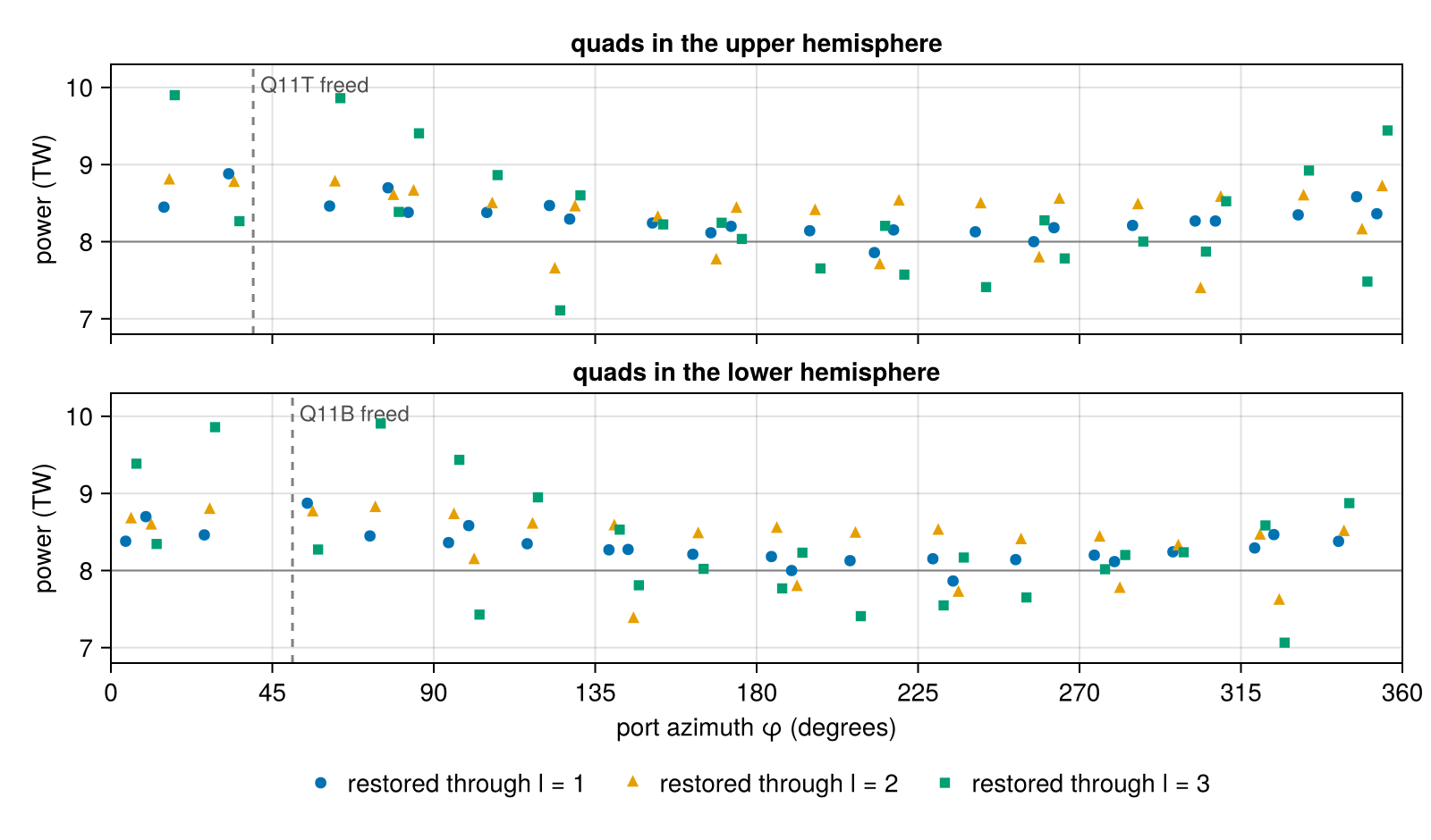
The same answer comes from the optimizer. optimize_pointing minimizes an objective of an Evaluation over the scenario's parameters, here the 46 quad powers, with gradients from forward-mode automatic differentiation. With the misfit of the $l \le 2$ coefficients as the objective and the bounds out of reach, L-BFGS-B starts from $P$ and moves only within the span of the gradients, which is the row space of $M_2$; it therefore converges to the minimum-norm solution:
power_only = subset(scenario, keep; parameterization = GroupPointing(remaining; by = :quad,
                                                                     fields = (:power,)))
misfit(ev) = sum(abs2, flux_ylm(ev; lmax = 2) .- full[1:9]) / full[1]^2
P0 = initial_parameters(power_only.param)
fit = optimize_pointing(power_only, misfit; x0 = P0, lower = fill(0.0, length(P0)),
                        upper = fill(20.0, length(P0)), g_tol = 1e-14)
@printf("misfit %.1e → %.1e,  max |P_optimizer − P_pseudoinverse| %.1e TW\n",
        fit.initial_value, fit.value, maximum(abs.(fit.x - rebalanced[2])))
misfit 1.5e-03 → 2.1e-24, max |P_optimizer − P_pseudoinverse| 2.2e-10 TWRemedy 3: re-point
Re-aiming quads moves drive around the hohlraum at no cost in power. Let each of the remaining quads move its aim by up to 0.3 mm along the hohlraum axis and sideways around it, and minimize mode 1 strongly and modes 2–4 weakly while holding the drive at its value after the bundle is freed. asymmetry_objective builds that objective and adds penalties for light clipped by the entrance holes and light striking the capsule. Each optimization here stops after a fixed number of L-BFGS-B iterations, 40 and then 20, short of full convergence but well past the point where mode 1 is gone.
repoint = subset(scenario, keep; parameterization = GroupPointing(remaining; by = :quad,
                                                                  fields = (:phi, :z)))
x0 = initial_parameters(repoint.param)
lower, upper = bounds(repoint.param, x0; phi = 0.3, z = 0.3)
goals = (modes = (1 => 200.0, 2 => 1.0, 3 => 1.0, 4 => 1.0), drive = c_free[1] / sqrt(4π),
         drive_weight = 10.0)
first_try = optimize_pointing(repoint, asymmetry_objective(; goals...); x0, lower, upper,
                              iterations = 40)
show_modes("bundle 11 freed", c_free)
show_modes("re-pointed", flux_ylm(evaluate(repoint, first_try.x); lmax = 4))
@printf("clipped %.1e of the delivered power\n", clipped_fraction(evaluate(repoint, first_try.x)))
bundle 11 freed ε₁ 1.080% ε₂ 15.267% ε₃ 0.786% ε₄ 0.710% drive 0.9625
re-pointed ε₁ 0.002% ε₂ 13.695% ε₃ 0.680% ε₄ 0.471% drive 0.9598
clipped 1.8e-07 of the delivered powerMode 1 is gone and nothing is clipped. But the clipping penalty sees only the nominal beams, and a shot review judges a pointing on its worst case. clearance grows each beam's envelope (here its contour at 1% of the peak, the level of LMF's target-configuration rules, spread by the f-cone) by 50 µm of pointing error and 25 µm of target positioning, adds ±1 mm of focus error, and reports the smallest distance to the end caps, together with the worst-case power and intensity the caps receive. The scattered-light wings, which reach the entrance-hole lip in any design, are left out:
function cap_review(beams)
    report = clearance(target, beams; targets = (:wall, :capsule),
                       hardware = (:cap_top, :cap_bottom), peak_fraction = 0.01, wings = [],
                       nangles = 8)
    return (nominal = minimum(r -> r.nominal, report.rows),
            worst = minimum(r -> r.clearance, report.rows),
            power = maximum(r -> r.intercepted, report.rows),
            fail = count(r -> r.status === :fail, report.rows))
end
review_line(label, r) = @printf("%-22s nominal %6.3f mm   worst case %6.3f mm   cap power ≤ %.1e   %d fail\n",
                                label, r.nominal, r.worst, r.power, r.fail)
review_48 = cap_review(quads)
review_line("48 quads", review_48)
review_line("re-pointed", cap_review(first_try.beams))
48 quads nominal 0.205 mm worst case 0.066 mm cap power ≤ 6.0e-08 0 fail
re-pointed nominal -0.017 mm worst case -0.155 mm cap power ≤ 7.0e-04 12 failThe original pointing clears the caps by 66 µm in the worst case. The re-pointed quads have used up that margin: in the worst case their 1% contours overlap the entrance-hole lips, several of them fail, and up to several times 10⁻⁴ of a beam's power lands on a cap.
The optimizer has to see the same worst case. An ApertureKeepOut computes each beam's worst-case clearance from the rim of its entrance hole with the same envelope and error set, smoothly enough to differentiate, and adds a penalty when it falls below a minimum, here 10 µm. On the original pointing it agrees with clearance:
keepout = ApertureKeepOut(target; peak_fraction = 0.01, minimum = 0.01, weight = 1e3)
from_keepout = aperture_clearance(keepout, quads)
@printf("worst-case clearance from the keep-out %.3f mm, from clearance %.3f mm\n",
        minimum(from_keepout), review_48.worst)

second_try = optimize_pointing(repoint, asymmetry_objective(; goals..., keepout); x0,
                               lower, upper, iterations = 20)
repointed = evaluate(repoint, second_try.x)
c_repointed = flux_ylm(repointed; lmax = 4)
show_modes("re-pointed, keep-out", c_repointed)
review_line("re-pointed, keep-out", cap_review(second_try.beams))
worst-case clearance from the keep-out 0.066 mm, from clearance 0.066 mm
re-pointed, keep-out ε₁ 0.023% ε₂ 14.408% ε₃ 1.085% ε₄ 0.671% drive 0.9600
re-pointed, keep-out nominal 0.153 mm worst case 0.014 mm cap power ≤ 7.1e-07 0 failRe-pointing within the clearance still removes nearly all of mode 1, to a few kilometres per second of hot-spot velocity, and the drive stays within 0.3% of its value after the bundle is freed. The worst-case clearance comes out at 14 µm rather than exactly the 10 µm asked for: the penalty is soft, and the keep-out's distance differs from the clearance check's by a few micrometres. The flux on the capsule before and after re-pointing, on the same maps and color scales as above:
fig = Figure(size = (800, 470))
for (j, (title, H, c)) in enumerate((("bundle 11 freed", H_free, c_free),
                                     ("re-pointed within clearance", repointed.flux, c_repointed)))
    capsule_panel(fig[1, j], deviation(H, c), 15; title)
    capsule_panel(fig[2, j], deviation(H, c) - deviation(H_full, full), 2)
end
Colorbar(fig[1, 3]; colormap = :balance, colorrange = (-15, 15), height = Relative(0.8),
         label = "H/⟨H⟩ − 1 (%)")
Colorbar(fig[2, 3]; colormap = :balance, colorrange = (-2, 2), height = Relative(0.8),
         label = "change from 48 quads (%)")
capsule_legend(fig[3, 1:2])
rowgap!(fig.layout, 6)
fig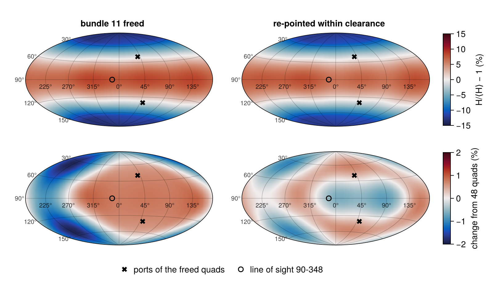
Re-pointing removes the warm side around the freed ports. What remains of the change from the 48-quad drive is in the higher modes, which the objective weighted two hundred times less than mode 1: the re-pointed drive trades the dipole for a stronger $l = 3$, while $l = 2$ is as it was with all 48 quads.
Independent check
The optimizer worked through the deposition operator and the linear flux response. raytrace_deposition recomputes the deposition of the re-pointed quads by tracing rays from each spot through its f-cone, and solve recomputes the radiosity directly:
traced = raytrace_deposition(target, second_try.beams; nspot = 61)
H = solve(scenario.model, traced).H[capsule]
show_modes("re-pointed, ray-traced", ylm_weights(target, capsule; lmax = 4) * H)
re-pointed, ray-traced ε₁ 0.029% ε₂ 14.408% ε₃ 1.078% ε₄ 0.667% drive 0.9598What this checks
- The NIF ports have the symmetry $D_2$ and no more, and every harmonic that $D_2$ forbids vanishes from the computed drive to round-off.
- Bundles in the same $D_2$ orbit cost the same in every mode, as the symmetry requires.
- Three routes to the drive without a bundle agree to round-off: a scenario on the remaining beams, the full scenario with the bundle at zero power, and the influence matrix.
- Freeing a bundle together with its image under the 180° rotation about the hohlraum axis removes mode 1.
- The power rebalance from the pseudoinverse and from the automatic-differentiation optimizer agree, as they must for a linear least-squares problem solved from the same start.
- The keep-out's worst-case clearance agrees with the clearance check's, and re-pointing against it passes that check.
- The re-pointed drive, recomputed by ray tracing and a direct radiosity solve, reproduces the optimizer's modes.
This page was generated using Literate.jl.