Pointing and power errors
No two shots point their beams the same way. Each NIF beam lands within about 50 µm (rms) of where it was aimed, and the beams' powers differ from their requests by a few percent. These errors are independent from beam to beam, so they do not cancel the way the symmetric design does: they leave a random low-mode asymmetry in the drive, and the mode-1 part of it, a flux difference between opposite sides of the capsule, displaces the hot spot (about 100 km/s per percent of mode-1 flux; MacGowan et al., High Energy Density Physics 40, 100944, 2021).
This tutorial computes how much asymmetry such errors leave in a NIF hohlraum's drive, checks the linear estimate against a Monte Carlo of full evaluations, and uses it to design a pointing that is less sensitive to the errors. It introduces mode_sensitivity, mode_uncertainty, sample_modes and the uncertainty keyword of the symmetry objectives.
using Briareus
using CairoMakie
using LinearAlgebra
using Printf
using Random
CairoMakie.activate!(type = "png", px_per_unit = 2)
set_theme!(fontsize = 15, linewidth = 2.5)
The hohlraum
The hohlraum and pointing of the Freeing a bundle for radiography tutorial: 10.1 × 5.75 mm with 3.1 mm entrance holes and a 0.9 mm capsule, 48 quads at 8 TW with their phase-plate spots, outer cones aimed on the axis near the entrance-hole planes and inner cones across the hohlraum. The mesh is coarser than the default to keep the tutorial quick.
target = hohlraum(length = 10.1, radius = 2.875, leh_radius = 1.55, capsule_radius = 0.9,
                  wall = gold(albedo = 0.85, conversion = 0.8), h = 0.45, capsule_h = 0.12)
p = GroupPointing(nif_quads(power = 8.0); fields = (:z, :r))
published = Dict(:outer50 => (5.01, 0.0), :outer44 => (5.20, 0.0),
                 :inner30 => (3.63, -0.60), :inner23 => (3.09, -1.09))
x0 = reduce(vcat, [[published[k]...] for k in p.keys])
quads = apply(p, x0)
scenario = Scenario(target, quads; observe = :capsule, parameterization = p,
                    viewfactor_kw = (; closed = true))
@printf("%d elements, %d quads\n", nelements(target), length(quads))
2736 elements, 48 quadsHow each beam's errors move the drive
Write the capsule's incident flux in real spherical harmonics, $c_{lm}$ (see the radiography tutorial), and its shape as $c_{lm}/c_{00}$. A beam's errors are its displacement transverse to the beam, along the two axes of its elliptical spot, and a fractional power error. Each beam's deposition depends on its own errors only, so mode_sensitivity differentiates every beam's contribution with three dual numbers in one pass, exactly. Against central differences of full evaluations:
lmax = 4
sens = mode_sensitivity(scenario, quads; lmax)
shape(bs) = (c = flux_ylm(evaluate(scenario, bs); lmax); c ./ c[1])
worst = 0.0
for (bi, k) in ((3, 1), (17, 2), (30, 3), (44, 1))
    b = quads[bi]
    e1, e2 = spot_axes(b)
    move(δ) = k == 3 ? remake(b; power = b.power * (1 + δ)) :
              remake(b; aim = b.aim + δ * (k == 1 ? e1 : e2))
    h = 1e-4
    fd = (shape([j == bi ? move(h) : quads[j] for j in eachindex(quads)]) .-
          shape([j == bi ? move(-h) : quads[j] for j in eachindex(quads)])) ./ 2h
    global worst = max(worst, maximum(abs, fd .- sens.J[:, 3(bi-1)+k]) / maximum(abs, fd))
end
@printf("largest relative difference from central differences: %.1e\n", worst)
largest relative difference from central differences: 2.2e-09The columns are the drive's response to each error. For mode 1, the pointing columns of the inner quads, whose spots land on the wall across from their ports near the waist, are the largest:
l1 = 2:4                                      # c_1,-1, c_10, c_11
per_beam(k) = [norm(sens.J[l1, 3(b-1)+k]) for b in eachindex(quads)]
for g in (:inner23, :inner30, :outer44, :outer50)
    idx = findall(b -> b.group === g, quads)
    @printf("%-8s |∂c₁/∂(pointing)| %.3f per mm, |∂c₁/∂(power)| %.3f per unit fraction\n", g,
            sum(per_beam(1)[idx] .+ per_beam(2)[idx]) / 2length(idx), sum(per_beam(3)[idx]) / length(idx))
end
inner23 |∂c₁/∂(pointing)| 0.008 per mm, |∂c₁/∂(power)| 0.011 per unit fraction
inner30 |∂c₁/∂(pointing)| 0.008 per mm, |∂c₁/∂(power)| 0.012 per unit fraction
outer44 |∂c₁/∂(pointing)| 0.003 per mm, |∂c₁/∂(power)| 0.009 per unit fraction
outer50 |∂c₁/∂(pointing)| 0.003 per mm, |∂c₁/∂(power)| 0.008 per unit fractionThe asymmetry the errors leave
With independent errors of rms size $\sigma_j$, the covariance of the shape is $J\,\mathrm{diag}(\sigma_j^2)\,J^\mathsf{T}$ to first order. mode_uncertainty takes the rms pointing as the length of the displacement ($\sigma/\sqrt 2$ along each axis) and the rms fractional power, and returns, for each degree $l$, the rms of $\sqrt{\sum_m (\delta c_{lm}/c_{00})^2}$, the share of mode $l$ the errors use up. For NIF's 50 µm pointing and a 3% power imbalance:
errors = (; pointing = 0.05, power = 0.03)
u = mode_uncertainty(scenario, quads; errors..., lmax)
for l in 1:lmax
    @printf("l = %d: rms %.3f%% of the mean flux\n", l, 100 * u.rms_mode[l])
end
pointing_only = mode_uncertainty(scenario, quads; pointing = 0.05, power = 0.0, lmax)
@printf("mode 1 from pointing alone %.3f%%, from power alone %.3f%%\n", 100 * pointing_only.rms_mode[1],
        100 * mode_uncertainty(scenario, quads; pointing = 0.0, power = 0.03, lmax).rms_mode[1])
l = 1: rms 0.279% of the mean flux
l = 2: rms 0.212% of the mean flux
l = 3: rms 0.131% of the mean flux
l = 4: rms 0.033% of the mean flux
mode 1 from pointing alone 0.199%, from power alone 0.196%The linear estimate holds while the errors are small against the spots' scale. A Monte Carlo of full evaluations, each with fresh random errors on every beam (sample_modes), is the independent check:
samples = sample_modes(scenario, quads; errors..., n = 300, lmax, rng = MersenneTwister(2026))
mc = [sqrt(sum(abs2, samples[l^2+1:(l+1)^2, :] .- u.c[l^2+1:(l+1)^2]) / size(samples, 2))
      for l in 1:lmax]
for l in 1:lmax
    @printf("l = %d: linear %.3f%%, Monte Carlo %.3f%% (ratio %.2f)\n", l, 100u.rms_mode[l],
            100mc[l], mc[l] / u.rms_mode[l])
end
l = 1: linear 0.279%, Monte Carlo 0.277% (ratio 0.99)
l = 2: linear 0.212%, Monte Carlo 0.207% (ratio 0.98)
l = 3: linear 0.131%, Monte Carlo 0.130% (ratio 0.99)
l = 4: linear 0.033%, Monte Carlo 0.033% (ratio 0.99)They agree to the sampling error of 300 shots, a few percent. The mode-1 amplitude over the samples, as a hot-spot velocity budget at 100 km/s per percent:
ε1 = [sqrt(3 * sum(abs2, samples[2:4, k])) for k in axes(samples, 2)]   # mode_amplitude
fig = Figure(size = (640, 330))
ax = Axis(fig[1, 1], xlabel = "mode-1 amplitude ε₁ (%)", ylabel = "shots",
          title = "Mode 1 from 50 µm pointing and 3% power errors")
hist!(ax, 100 .* ε1; bins = 30, color = (:steelblue, 0.8))
vlines!(ax, [100 * sqrt(3) * u.rms_mode[1]]; color = :black, linestyle = :dash)
fig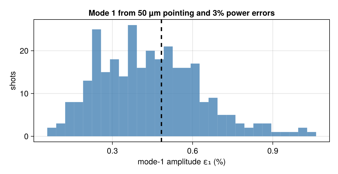
@printf("ε₁: median %.2f%%, 90th percentile %.2f%% (≈ %.0f km/s); linear rms √3 × %.3f%% = %.2f%%\n",
        100 * sort(ε1)[end÷2], 100 * sort(ε1)[9end÷10], 100 * 100 * sort(ε1)[9end÷10],
        100 * u.rms_mode[1], 100 * sqrt(3) * u.rms_mode[1])
ε₁: median 0.43%, 90th percentile 0.67% (≈ 67 km/s); linear rms √3 × 0.279% = 0.48%Does the pointing change the budget?
The errors' share of each mode depends on where the spots land: a spot on a steep part of the drive's response moves the shape more for the same displacement. First tune the cones (aim and power per cone, aims within 1.5 mm axially and 1 mm radially, powers within 40%) to null $l = 1$–$4$ at fixed drive, and compare the budgets of the published and the tuned designs:
p3 = GroupPointing(quads; fields = (:z, :r, :power))
s3 = Scenario(target, quads; observe = :capsule, parameterization = p3,
              viewfactor_kw = (; closed = true))
x3 = initial_parameters(p3)
a0 = flux_moments(evaluate(s3, x3))[1]
lo, hi = bounds(p3, x3; z = 1.5, r = 1.0, power = 0.4)
keepout = (ApertureKeepOut(target), SphereKeepOut(target))
modes = (1 => 1.0, 2 => 1.0, 3 => 1.0, 4 => 1.0)
tuned = optimize_pointing(s3, symmetry_objective(; modes, odd = 0.0, drive = a0, keepout);
                          x0 = x3, lower = lo, upper = hi, iterations = 200)
function budget_row(label, x)
    ev = evaluate(s3, x)
    a = flux_moments(ev; lmax = 4)
    ur = mode_uncertainty(s3, ev.beams; errors..., lmax)
    @printf("  %-10s %+7.3f%%  %+7.3f%%          %s
", label, 100a[3] / a[1], 100a[5] / a[1],
            join((@sprintf("%.3f%%", 100x) for x in ur.rms_mode), "  "))
    return ur.rms_mode
end
println("  design      P₂/P₀     P₄/P₀    rms from the errors: l = 1     2      3      4")
budget_row("published", x3)
tuned_budget = budget_row("tuned", tuned.x);
design P₂/P₀ P₄/P₀ rms from the errors: l = 1 2 3 4
published -14.547% +0.322% 0.279% 0.212% 0.131% 0.033%
tuned -0.019% +0.077% 0.233% 0.157% 0.090% 0.021%The tuned design leaves less to the errors (l = 1 from 0.28% to 0.23%). It has also moved power from the inner cones, whose errors weigh most per beam (above), to the outer ones. With uncertainty, symmetry_objective minimizes instead the expected value of each mode's square over the errors, the nominal value plus the variance they add (at about three times the cost per evaluation, through nested dual numbers). Started from the tuned design:
robust = optimize_pointing(s3, symmetry_objective(; modes, odd = 0.0, drive = a0, keepout,
                                                  uncertainty = errors);
                           x0 = tuned.x, lower = lo, upper = hi, iterations = 30)
robust_budget = budget_row("robust", robust.x)
@printf("largest change of a cone parameter: %.3f; of the l = 1 budget: %+.1f%%
",
        maximum(abs, robust.x .- tuned.x), 100 * (robust_budget[1] / tuned_budget[1] - 1))
robust -0.019% +0.077% 0.233% 0.157% 0.090% 0.021%
largest change of a cone parameter: 0.000; of the l = 1 budget: -0.0%The robust objective barely moves the tuned design: within these bounds, where the cones point hardly changes how much asymmetry independent beam errors leave. They set a floor, about a quarter of a percent of mode 1 here, that only better pointing accuracy and power balance lower.
What this checks
- The per-beam sensitivities from dual numbers match central differences of full evaluations (printed above; the test suite checks them to 1e-6).
- The linear propagation of independent errors matches a Monte Carlo of full evaluations to its sampling error, mode by mode.
- The robust objective adds exactly the propagated variance to the nominal one (test suite), and its gradients, through nested dual numbers, match finite differences.
This page was generated using Literate.jl.